Update 3
Overview
After update 1 and 2, we have been working on connecting the more independent explorations and progress we have made to get closer to our main goal of correlating pH with larval fish abundance. We have stepped beyond the inital exploratory aspects of the project and have completed data processing, began exploring species correlations, and looked further into kriging for data interpolation. With our calculations of pH, we are beginning to explore its relationship to the species and other factors in our datasets.
Reiterating Our Project and Goal
In our project, we aim to correlate water data containing many water characteristics at a given location and time, to our fish data, in order to draw better understand relationships between how water characteristics affect the makeup of specific species in California’s oceans. We are especially interested in seeing how water pH affects the makeup of these fish species. We hope that our conclusions can be used to for one, be able to accurately infer what the makeup of fish looks like at a given time where we know the water makeup, and two also be able to predict what the makeup of fish should look like in the future. We hope that this will help reduce the effort needed to be able to get a portrayal of the makeup of fish, since currently usually sampling the fish by a boat all along California’s oceans is the effort that is needed.
We are have a water time series dataset, what gives information about many water characteristics over many different locations, from 2008-2015, and we also have a fish time series dataset that tells us the abundance of each fish species at a given location and time, from the 1960’s until present.
Data Processing
Adding pH Calculations to Fish and Water Data
Data processing has been a big part of this project as we have to connect the water characterisitcs data to the larval fish data. After subsetting the larger fish dataset to match the avaialble dates and locations from the water data, we were able to match fish and water observations and added in the calculated pH values for each observation, as mentioned in Update 2. Being able to have the pH for each observation was a huge step towards our main project goal of correlating pH to larval fish abundance. Now we have all variables and measurements in one dataset with matching dates and locations from water, fish and pH calculations. We then decided to remove the water characteristics, except salinity and temperature. Because these water characteristics were used in the calculation of pH, we can infer their relationship with the species’ abundance through their relationship with pH and we mostly care about pH for the purpose of this project to observe the effects of climate change.
Relative Abundance
The original larval fish dataset gave an abundance measurement for each species. For the sake of this project we want to look at how the abundance is changing over time so we wanted a abundance value that would allow us to do that among species. With current measurement, we are not able to compare values with other species to see which are increasing more or less relative to each other. To solve this issue, we calculated a “relative abundance” value within each species using the formula:
(value - average abundance) / average abundance
We changed all 0 values (where there is no observation of a species) to NA values so that we could distinguish it with an abundance observation that is equivalent to the mean, meaning a relative abundance of 0.
Formatting Datasets
One issue we ran into with the way the datasets differed was that the water dataset was collected in the same locations over different depths while the fish dataset only had one collection per location. pH was calulated using the water characteristics at each depth so for one location their were multiple pH values. To avoid having repeated fish adundances, we found the minimum, maximum and mean pH values over the depths for each location. This allows us to keep some of the integrigity of the water dataset but also make it flow easily with the larval fish data.
Seeing that we had a very wide dataset (large number of columns), we created a long (more rows, less columns) format dataset. This would make it easier to filter the dataset to subset a particular species or pH measurement (min, max, or mean) to explore. To do this, we created a column for the species name, relative abundance, pH measurement, and pH value.

Fig. 8 Wide Dataset: This is the format of the data after water, fish, and pH were combined into one dataset and the min, max and mean pH values are calculated.
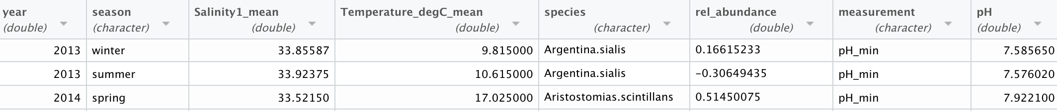
Fig. 9 Long Dataset: This is the format of the “long” dataset with the pH and abundances turned into columns.
Cluster Network
Now that we calculated the pH balances and the relative fish abundance we want to look at the pairwise correlation between each fish species relative abundance and their pH values associated with them. We were able to make a correlation matrix that uses the method of perasons r to find pairwise correlation and used a heat map to visualize the correlation matrix created.The side bar color ranges the pearsons r coefficient with the color being close to 1 range is strong positive and and -1 is a strong negetive relationship and 0 signifying no correlation.
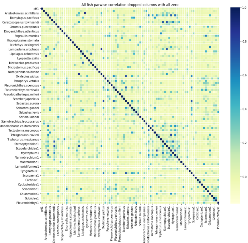
Fig. 10 Heat map: This is the heatmap of the correlation matrix we created that founded pairwise correlation using pearsons r method.
From here I was able to use the hierarchical cluster method to find a cluster network. With the clustering founded I was able to visualize it with the sides repesenting the dendogram of the clustering along with the heat map of the correlation network founded like the image above explained.The image below is the clustering network founded.
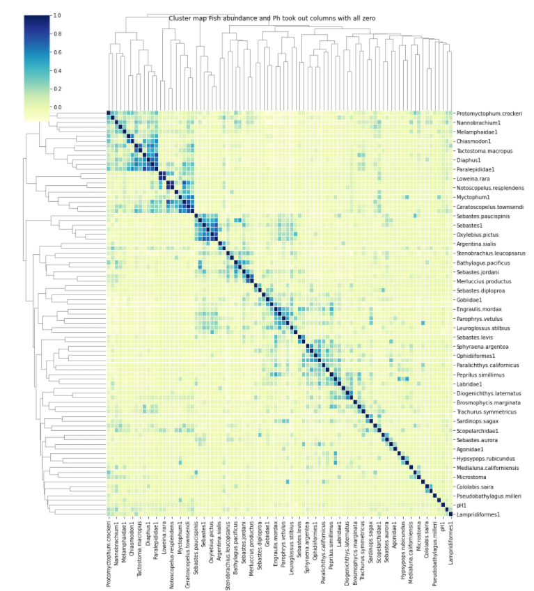
Fig. 11 Cluster network: This is the clusters we founded using hierachal clustering and also includes the heat map to shows the pairwise correlation between each species relative abundance and its pH value.
The visualization above will give us a better understanding of the relationship between each fish species relative abundance and their pH values. This anaylsis is still ongoing and will explain significiance of the visualization in greater detail in the next progress report.
Kriging
We are currently working on the process of using Kriging on some of our data, which is a method of interpolation. For example, we have the values of water characteritics, say pH, at discrete stations in the water, and we would like to infer what the pH should be in between those stations as well. To do this, we intend to use a process called cringing to do this for all of our water characteritics. We are currently working on solving the challenge of turning our data from our stations that we would like to perform Kriging on and turn it onto square shaped data for the Kriging algorithm.
This challenge arises because right now, our stations are aligned in a slanted way since they are off of California’s coast, and at every time step that we want to do Kriging on, we do now have the same number of samples, and the number of samples differ for each water characteristic as well. This makes turning the data into a square matrix difficult, so we are looking at two different methods right now to achieve this: using 2-D histograms as well as Voronoi Tesselations (two methods that help in evening out data in a matrix form acceptable for Kriging). We hope to use this method to format our data correctly to succesfuly apply the Kriging algorithm to our data.
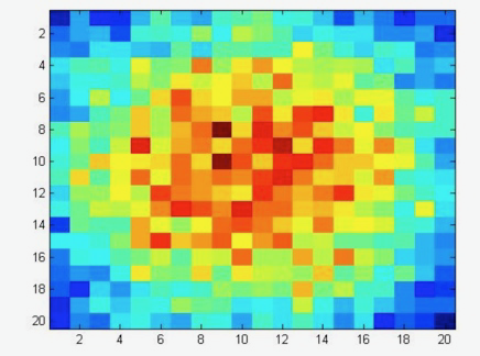
Fig. 12 An example of A 2D histogram from MathWorks.com. This is not our 2D histogram, but with this we hope to illustrate the purpose of the 2D histogram. We seen by the image, the 2D histogram aggregates the data, which would be the samples taken in our case for a particular water characteristic at a time step, in a small area and does this to return a square/grid matrix of samples.
Out Next Future Goals
As our next goals, we hope to complete our Kriging process as well as keep drawing stronger correlations between how the fish species behave between each other (which are more abundant at the same time, and are there species who are abundant at opposite times of each other), as well as between how pH and dictate which fish species will be abundant and which will not be at a time and location in the water. We have ample data analysis, and different insights about various parts of our data currently. In order to work towards achieving ths goal, we hope to keep working on putting these insights and different parts of our project together as well as draw further insight from what we have now, in order to achieve our previously stated goal. We find that often we have been gaining more and more insight by looking at multiple parts of our current findings, and trying to observe how these findings are relating to each other. This helps us discover new relationships, and we hope to keep proceeding this way in order to find the correlations we ultimately want.